
“Antivirus is dead” is a common refrain in the information security space, but if you look below the surface, what it really means is “atomic indicators are dead.” While there is value in static indicators, they are the bare minimum standard for detection these days and suffer from numerous drawbacks. Behavioral indicators are the next level, which use knowledge of adversarial techniques to find both known and unknown activity. This is the category entropy falls into: looking at a known technique (randomized data to thwart atomic indicators) to find both known and unknown malware.
In this article, we’ll dig into the possibility of using entropy in threat hunting to help identify adversarial behavior. I’ll first explain what is typically meant when people talk about entropy (Shannon entropy) before moving on to a similar formula (relative entropy) which has better applications in information security. I will then show how relative entropy can be utilized against letter frequency patterns in domain names to identify malicious ones. Because some families of malware use domain generation algorithms that change domains frequently, blacklisting these types of domains is not an efficient means to protect environments.
Ready? Let the math begin…
What Is Entropy?

If you have worked in InfoSec for long, you have no doubt heard the term entropy. Furthermore, you are probably familiar with Shannon entropy and how it is used to measure randomness. While this term is probably not new to you, the meaning of entropy depends on the context in which it is used. In the context of digital information, entropy—specifically information entropy—is typically thought of as a measure of randomness or uncertainty in data.
A Brief History of Entropy

The term entropy was first used in thermodynamics, the science of energy, in the 1860s. It wasn’t until 1948 that the concept was first extended to the context we are interested in. In that year, Claude Shannon published the famous paper A Mathematical Theory of Communication, which defined the field of information theory and, among other things, the idea of information entropy. Since then, entropy has found many uses in different aspects of modern digital systems, from compression algorithms to cryptography.
The Formula
This is the formula for calculating information entropy:

At first glance this looks fairly complex, but after defining the terms involved it becomes much less mysterious. In the formula above:
- H is the symbol for entropy, and X is the input data, so H(X) means “The entropy of data X.”
- The sigma (
 ) represents a summation that sums up
  for values from i = 1 to n. Think of summation as a loop which iterates over each unique character in a string.
The part inside the summation ![]() is the most important part of the equation, because this is what assigns higher numbers to rarer events and lower numbers to common events. pi represents the proportion of each unique character i in the input X. For example, in the message “Hello”:
is the most important part of the equation, because this is what assigns higher numbers to rarer events and lower numbers to common events. pi represents the proportion of each unique character i in the input X. For example, in the message “Hello”:
- pH = 0.2 because “H” was observed 1 time in 5 characters, and 1 / 5 = 0.2.
- pe = 0.2 and po = 0.2.
- pl = 0.4 since there are two observed “l”s.
If you recall, I mentioned that common events get lower values, but in the “Hello” example, the most common character has the highest value, and this is where the logarithm comes in.
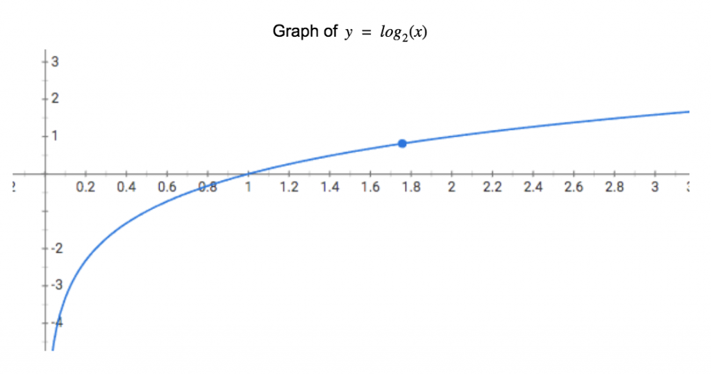
Above is a graph of the base-2 logarithmic function, which illustrates two key points of the original equation. First, we can see why the equation has a negative sign before the summation. Because ![]() will never be greater than 1 (a proportion can never be more than 1, because even in the message “aaa”,
will never be greater than 1 (a proportion can never be more than 1, because even in the message “aaa”, ![]() ), the value of
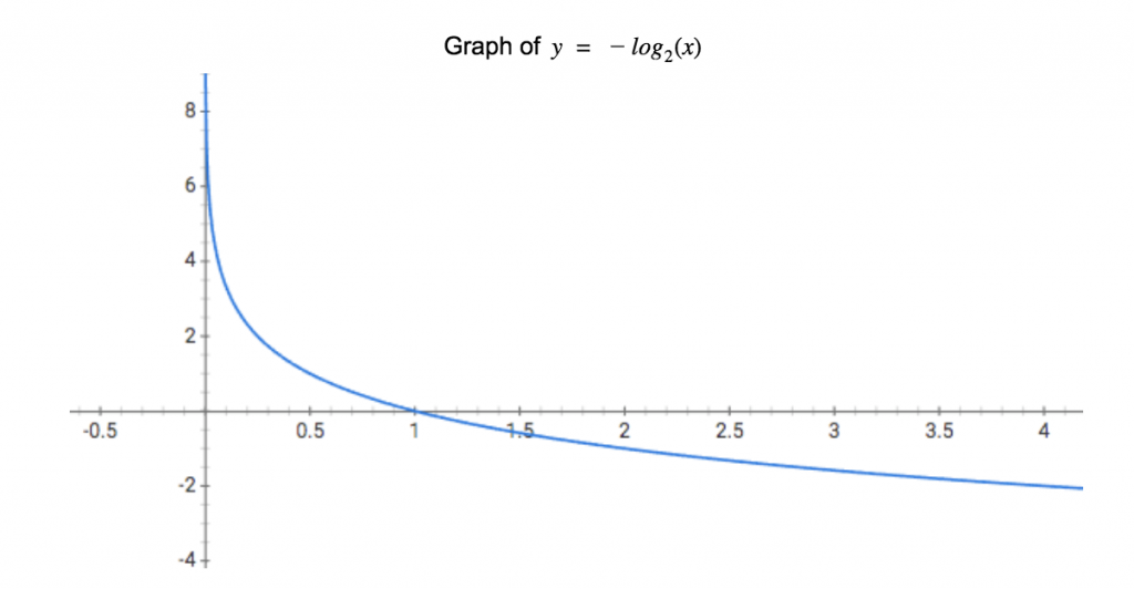
), the value of ![]() will always be negative. If we invert the graph, we can now clearly see that as
will always be negative. If we invert the graph, we can now clearly see that as ![]() approaches 1 (becomes more common in the data),
approaches 1 (becomes more common in the data), ![]() approaches 0.
approaches 0.
To summarize, the formula is equal to the negative of the sum of the proportion of i multiplied by the logarithm of the proportion of i.
One more important aspect to note is the base of the logarithm used, which represents the number of symbols available to use when representing the message. The most common base is 2, since most applications of entropy deal with binary data (bits), where only 0 and 1 are available.
What Is Information Entropy?

The technical definition of information entropy (according to Wikipedia) is: “…the average amount of information produced by a probabilistic stochastic source of data.” In other words, it is the amount of information needed to represent the outcome of a random variable. In this way, it is a bit easier to see how entropy can be thought of as a measure of randomness or uncertainty.
A common example is that of a coin toss. A fair coin toss assumes that both heads and tails are equally likely, so each outcome has a 50% probability of occurring. Because there are two possible outcomes, the result of each toss can be thought of as a bit (0 = heads, 1 = tails), and a sequence of tosses can be represented as a binary sequence. Since each outcome is equally likely, the minimum amount of information needed to represent each outcome is also one bit. This is because the outcome of each fair toss cannot be predicted in advance, it can only be known after the toss has occurred.

If we consider an unfair toss, in which heads is 100% probable, each outcome requires 0 bits of information to represent. Because the outcome is certain, no new information is gained from each toss of the coin. In this situation, the outcome is entirely predictable in advance, and flipping the coin once, ten times, or one million times will not produce a different result.
In the coin toss example, the base of the logarithm would be 2 because there are two possible outcomes; heads and tails. Take a data compression algorithm as a second, more complex, example.
In this case, suppose the algorithm is attempting to encode a message comprised of the four directions “Up”, “Down”, “Left”, and “Right” as concisely as possible. A simple message to encode could be “Up”, “Up”, “Down”, “Down”, “Left”, “Right”, “Left”, “Right”. Each direction occurs equally in this message (p = 0.25), and our logarithm (-log2(0.25) = 2.0) tells us we would need 2 bits to encode each direction. We can confirm this by working it out, and if you are familiar with binary it probably wouldn’t take you any time at all to come up with:
- “Up” = 00
- “Down” = 01
- “Left” = 10
- “Right” = 11
Relative Entropy
Shannon entropy works well for detecting truly randomized data because it is the opposite of repetitive data. But what if you are trying to compare random data to data with another distribution, like the distribution of letters in English text? In a random string of letters, each letter should occur roughly equally, but in normal language, some letters are more common than others. A string of random letters differs from standard text in two ways: an underrepresentation of common letters (like ‘e’, ‘r’, ‘s’, and ‘t’), and an overrepresentation of uncommon letters (like ‘z’ and ‘q’).
Shannon entropy does not have a way to compensate for this; for example, in the string ‘microsoft’ every letter is repeated only once aside from ‘o’, which would make it appear that this string is highly random and that ‘o’ is the most common letter. This is where relative entropy comes in. It compares two distributions; in our case the distribution of English characters and a potentially malicious random string.
Naturally, there are a few differences between Shannon and relative entropy, and the formula for relative entropy is slightly different:
![]() You are probably wondering what the
You are probably wondering what the ![]() stands for, so I should take a moment to explain that relative entropy is also known as the Kullback-Leibler divergence because it was introduced in 1951 by Solomon Kullback and Richard Leibler. It is called a divergence because it measures the way two probability distributions diverge, but for simplicity and consistency I will refer to this as relative entropy.
stands for, so I should take a moment to explain that relative entropy is also known as the Kullback-Leibler divergence because it was introduced in 1951 by Solomon Kullback and Richard Leibler. It is called a divergence because it measures the way two probability distributions diverge, but for simplicity and consistency I will refer to this as relative entropy.
I won’t rehash everything I explained above, but there are some new elements in this formula. The biggest difference is that we now have two distributions, P and Q, and corresponding proportions for each: ![]() and
and ![]() . For our purposes, Q will be the baseline distribution, calculated on a set of legitimate data, and P will be the distribution in question (like a potentially malicious domain). The most important difference is the ratio in the logarithm. This is how we actually account for the difference in the distributions.
. For our purposes, Q will be the baseline distribution, calculated on a set of legitimate data, and P will be the distribution in question (like a potentially malicious domain). The most important difference is the ratio in the logarithm. This is how we actually account for the difference in the distributions.
First consider a distribution where ![]() and
and ![]() are equal; in this case, the logarithm would be of 1, which is 0. If both distributions are equal, then the summation would be a total of a bunch of 0s. Next, consider when they are unequal, if
are equal; in this case, the logarithm would be of 1, which is 0. If both distributions are equal, then the summation would be a total of a bunch of 0s. Next, consider when they are unequal, if ![]() is larger than
is larger than ![]() , then the logarithm will be larger than 1, and the total will increase. Conversely, if
, then the logarithm will be larger than 1, and the total will increase. Conversely, if ![]() is smaller than
is smaller than ![]() , then the logarithm will be smaller and will lower the total.
, then the logarithm will be smaller and will lower the total.
Using Relative Entropy
As I just stated, relative entropy compares TWO distributions, so to perform the calculations some baseline data needs to be collected. While this requires additional work, it improves the fidelity of the randomness detection. To detect randomly generated domain names, a common method for identifying malware using domain generation algorithms, you can use something like the Alexa top one million domains to build the following character frequency distribution:
DOMAIN_CHARACTER_FREQUENCIES = {
'-' => 0.013342298553905901,
'_' => 9.04562613824129e-06,
'0' => 0.0024875471880163543,
'1' => 0.004884638114650296,
'2' => 0.004373560237839663,
'3' => 0.0021136613076357144,
'4' => 0.001625197496170685,
'5' => 0.0013070929769758662,
'6' => 0.0014880054997406921,
'7' => 0.001471421851820583,
'8' => 0.0012663876593537805,
'9' => 0.0010327089841158806,
'a' => 0.07333590631143488,
'b' => 0.04293204925644953,
'c' => 0.027385633133525503,
'd' => 0.02769469202658208,
'e' => 0.07086192756262588,
'f' => 0.01249653250998034,
'g' => 0.038516276096631406,
'h' => 0.024017645001386995,
'i' => 0.060447396668797414,
'j' => 0.007082725266242929,
'k' => 0.01659570875496002,
'l' => 0.05815885325582237,
'm' => 0.033884915513851865,
'n' => 0.04753175014774523,
'o' => 0.09413783122067709,
'p' => 0.042555148167356144,
'q' => 0.0017231917793349655,
'r' => 0.06460084667060655,
's' => 0.07214640647425614,
't' => 0.06447722311338391,
'u' => 0.034792493336388744,
'v' => 0.011637198026847418,
'w' => 0.013318176884203925,
'x' => 0.003170491961453572,
'y' => 0.016381628936354975,
'z' => 0.004715786426736459
}
Now that we have collected our Q distribution we can compare another distribution (P) to it. It should be noted that although the distribution listed above was calculated on the Alexa top one million, all top level domains, label separators (.), and any occurrences of "www" were removed. Thus, a domain appearing as “en.www.wikipedia.org” would be reduced to “enwikipedia”. The idea behind this was to try remove some irrelevant data from the distribution, so when examining a randomized domain like “www.ywkejfh.com” the level of randomness would not be decreased by the presence of incredibly common labels like “www” or “com”. This isn’t perfect (what about“www2”?), but is adequate to get good results.
Speaking of results… let’s see how relative entropy compares to Shannon entropy. The best way to illustrate this is with a couple of graphs. (Because everyone loves graphs, right?)
Histogram of Alexa Top 1,000,000
The following diagram shows the distribution of Shannon and relative entropy values calculated for the Alexa top one million domains:
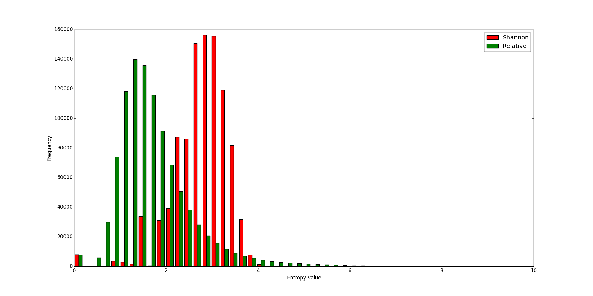
You can see that although there is a good bit of overlap, the relative entropy values on the horizontal axis are, on the whole, much lower than the Shannon entropies.
Now let’s look at the same chart, where this time the values were calculated for a small set of known malicious domains:
Histogram of a Sample of Malicious Domains
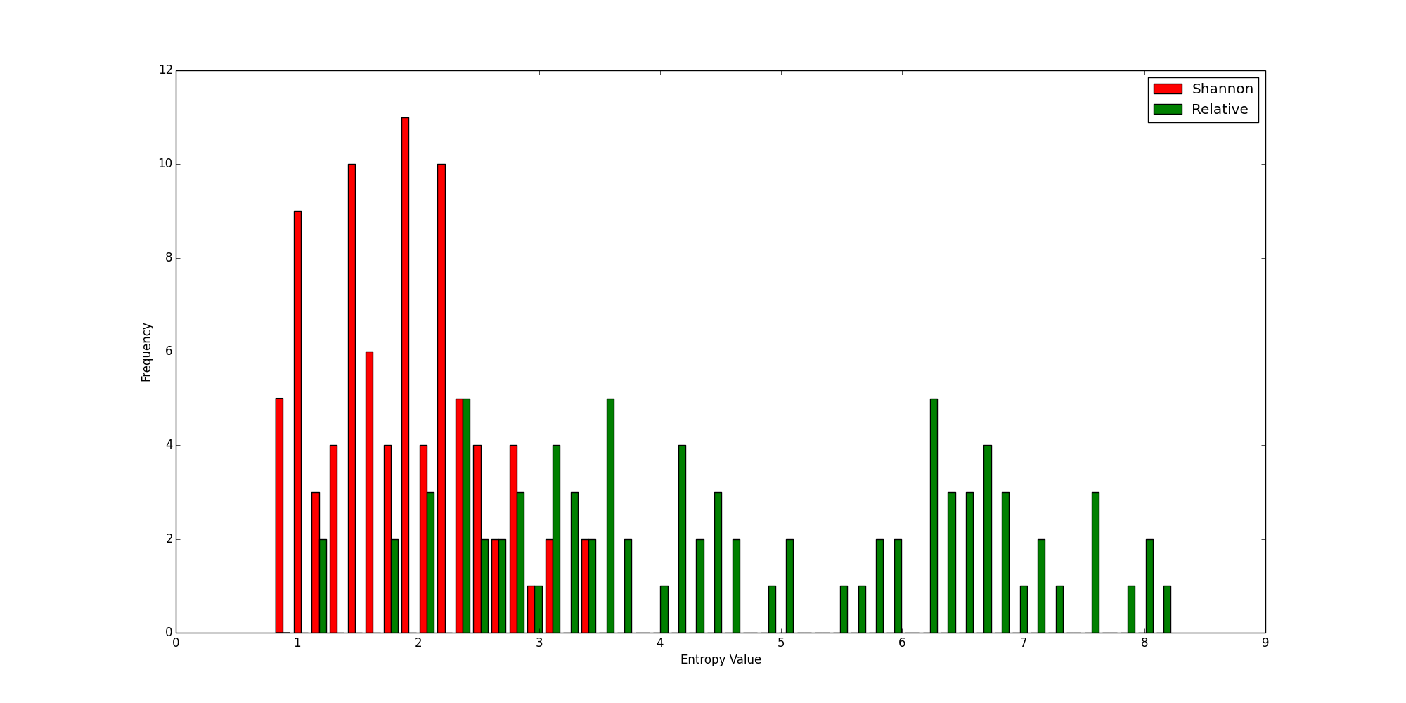
Again, there is some overlap, but this time the relative entropy values are generally higher than their Shannon counterparts. Combined with the previous chart, you can begin to see the power of relative entropy. The legitimate domains have lower scores, while the malicious ones have higher scores, so the distinction between legitimate domains and malicious domains becomes clearer. Because there is better separation between the good and the bad, it is easier to use a threshold to determine whether something is good or not, which is the main way entropy calculations are used. (I.e., is entropy greater than x?)
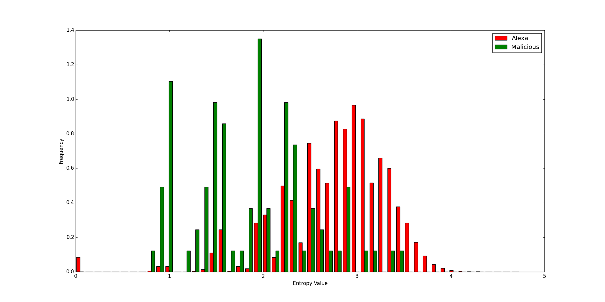
To further illustrate this point, let’s look at two more histograms showing the Shannon and Relative entropies calculated for every domain, color coded by legitimacy.
Shannon Entropies for Legitimate and Malicious Domains
 Relative Entropies for Legitimate and Malicious Domains
 Relative Entropies for Legitimate and Malicious Domains
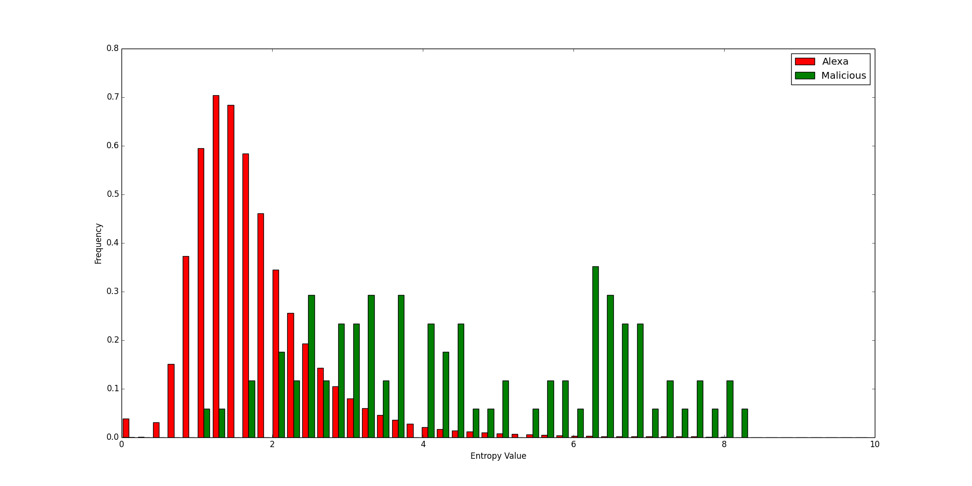
It should be clearly visible that the relative entropy better separates the good domains from the bad. While it is certainly not perfect, it outperforms the traditional Shannon entropy for this usage.
How the Heck Does This Help With Threat Hunting?
If you’ve made it this far, you are probably thinking, “This is all fine and dandy, but how is it useful? I clicked on this post because it said ‘threat hunting,’ not mathematics lesson!” And you are certainly justified in those thoughts; I’ve laid over 2000 words of foundation with little in the way of practical application.
But the larger the foundation, the taller you can build—and now we have plenty to build on.
The most obvious application at this point is to look for randomized domain names. Some families of malware use domain generation algorithms (DGAs) in an attempt to evade traditional detection techniques. You can’t blacklist a domain that changes hourly. (Well, you can, but it’s not going to be very effective.)

There are tools available that can create Windows services with random service names and descriptions. Numerous malware families also create registry keys for persistence with randomized key names and values. One last example is process names; often malware will put itself, randomly named, into a randomly named folder in AppData. There are actually two potential applications here: one for the name of the binary itself, and one for the randomly named folder in which it resides.
For each of these examples, or any other applications of relative entropy you can think of, there is a bit of overhead work which must be done. The first part is collecting and analyzing the data you are interested in. If you want to look for malicious process names, you will need to collect and count frequencies for characters which appear in a sample of process names (the larger the sample size, the better). Once you have collected this data, you must find a threshold which reduces false positives as much as possible while including as much malicious activity as possible. This metric will never be 100% reliable, but as I have shown, it can be much more effective to use relative entropy than Shannon entropy.
 There are ways to improve the performance of relative entropy when using it for detection. For many uses, it can be combined with other suspicious characteristics increase confidence in a signature. For example, you could look for an unsigned binary which makes a network connection to a domain with relative entropy over a certain threshold. Or a suspicious network connection made by a binary located in AppData. Red Canary does exactly this, looking for unsigned binaries located in AppData which make network connections made to domains with a relative entropy above 3.0.
All of these techniques can be used in a threat hunting program. We have taken an adversary’s technique, using randomized data to thwart static indicators, and developed our own technique for detecting said behavior. Our method is not based on any static indicator used by an adversary, but rather is looking for a symptom of a technique—such as something that appears random, but isn’t. Since the focus here is based on a broad behavior, any malware which uses this behavior would be detected, including both known and unknown families. This is the essence of threat hunting.
Key Takeaways
As I have outlined above, relative entropy can be an effective tool for rooting out evil. While it is not a silver bullet alone, it can be combined with other factors to improve its effectiveness. There are other methods for identifying random domain names (like n-gram analysis, usually with bigrams/digrams), but I hope that this blog serves as a starting point for further research into its potential applications in the information security industry.
Read more from this author: How to Use Windows API Knowledge to Be a Better Defender
'''
This module is for calculating various entropy measurements on two pieces of data.
'''
from __future__ import division
from collections import Counter
import math
__version__ = '0.1'
class Entropy(object):
'''
This class contains all of the entropy functions.
'''
def __init__(self, data=None):
self.data = data
# The various algorithms are stored in a class dictionary so all
# supported algorithms can be iterated through.
# See the calculate function for an example.
self.algorithms = {
# 'Hartley': self.hartley_entropy,
'Metric': self.metric_entropy,
'Relative': self.relative_entropy,
# 'Renyi': self.renyi_entropy,
'Shannon': self.shannon_entropy,
# 'Theil': self.theil_index,
}
def calculate(self, data):
'''
Calculate all supported entropy values
'''
results = {}
for algo in self.algorithms:
results[algo] = self.algorithms[algo](data)
return results
def metric_entropy(self, data, base=2):
'''
Calculate the metric entropy (aka normalized Shannon entropy) of data.
'''
entropy = 0.0
if len(data) > 0:
entropy = self.shannon_entropy(data, base) / len(data)
return entropy
def shannon_entropy(self, data, base=2):
'''
Calculate the Shannon entropy of data.
'''
entropy = 0.0
if len(data) > 0:
cnt = Counter(data)
length = len(data)
for count in cnt.values():
entropy += (count / length) * math.log(count / length, base)
entropy = entropy * -1.0
return entropy
def relative_entropy(self, data, base=2):
'''
Calculate the relative entropy (Kullback-Leibler divergence) between data and expected values.
'''
entropy = 0.0
length = len(data) * 1.0
if length > 0:
cnt = Counter(data)
# These probability numbers were calculated from the Alexa Top
# 1 million domains as of September 15th, 2017. TLDs and instances
# of 'www' were removed so 'www.google.com' would be treated as
# 'google' and 'images.google.com' would be 'images.google'.
probabilities = {
'-': 0.013342298553905901,
'_': 9.04562613824129e-06,
'0': 0.0024875471880163543,
'1': 0.004884638114650296,
'2': 0.004373560237839663,
'3': 0.0021136613076357144,
'4': 0.001625197496170685,
'5': 0.0013070929769758662,
'6': 0.0014880054997406921,
'7': 0.001471421851820583,
'8': 0.0012663876593537805,
'9': 0.0010327089841158806,
'a': 0.07333590631143488,
'b': 0.04293204925644953,
'c': 0.027385633133525503,
'd': 0.02769469202658208,
'e': 0.07086192756262588,
'f': 0.01249653250998034,
'g': 0.038516276096631406,
'h': 0.024017645001386995,
'i': 0.060447396668797414,
'j': 0.007082725266242929,
'k': 0.01659570875496002,
'l': 0.05815885325582237,
'm': 0.033884915513851865,
'n': 0.04753175014774523,
'o': 0.09413783122067709,
'p': 0.042555148167356144,
'q': 0.0017231917793349655,
'r': 0.06460084667060655,
's': 0.07214640647425614,
't': 0.06447722311338391,
'u': 0.034792493336388744,
'v': 0.011637198026847418,
'w': 0.013318176884203925,
'x': 0.003170491961453572,
'y': 0.016381628936354975,
'z': 0.004715786426736459
}
for char, count in cnt.items():
observed = count / length
expected = probabilities[char]
entropy += observed * math.log((observed / expected), base)
return entropyRelated Articles
Privilege escalation revisited: webinar highlights
Detection Déjà Vu: a tale of two incident response engagements
Detection Déjà Vu: a tale of two incident response engagements
Black Hat: Detecting the unknown and disclosing a new attack technique